Creating Irrigation Zones using Bayesian Neural Networks
 Photo by Yulian Alexeyev on Unsplash
This project was my Master’s project at BYU with the help of Dr. Matthew Heaton and Dr. Neil Hansen. I will provide many of the details, but some information as well as references will not be included here. We have a paper that is submitted for review currently. When it is published, the article title and the journal it is published it will be provided. Until this happens, if you are interested in further detail about the project, feel free to contact me and I can share what I have currently before it is published.
This project is longer than most of my projects because of the many different technical parts and it represents two years of work as well.
Background
The management of agricultural fields (i.e. farming) in the era of data science has evolved to use spatial mapping, remote sensing, soil and terrain measurements, weather measurements and other data sources to improve the quantity and quality of crops. The access to rich amounts of data provides opportunities for analysis that can inform decision making such as the amount of water and fertilizer to apply at any given time at any given location. The management of agricultural fields using advanced data analytics is referred to, collectively, as precision agriculture. Broadly, precision agriculture attempts to use the spatial variability within a field to manage individual crop locations rather than treat a field as spatially and temporally homogeneous. Given that agriculture fields often occupy multiple acres of space, precision agriculture has been shown to outperform basic farming techniques by increasing crop yield.
Crop yield is heavily driven by the volumetric water content (VWC; the ratio of the volume of water to the unit volume of soil) and, in arid regions, irrigation is a practiced method for controlling and adjusting the VWC. As such, variable rate irrigation (VRI) is a practice within precision agriculture focused on using data to adjust the amount of water applied throughout the field according to spatial and temporal variations. One approach to VRI is to partition the field into management zones (or irrigation zones) wherein irrigation rates are adjusted within each management zones rather than utilizing a constant irrigation rate throughout the entire field
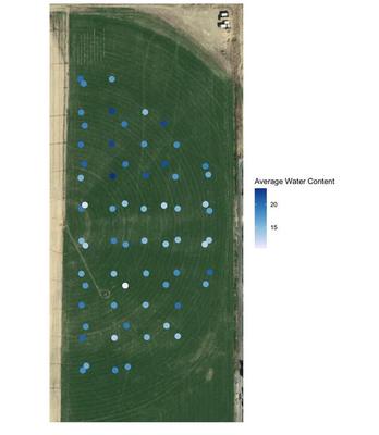
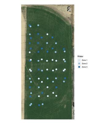
Effective irrigation zones should partition the agricultural field based on VWC. However, obtaining VWC is a labor intensive process and is often only sparsely measured for the entire field. As an example, Figure 1 below shows 66 VWC measurements averaged over four time periods between April and September 2019 for an agricultural field of winter wheat in Rexburg, Idaho. Although the VWC was recorded at 66 different locations, the available data do not adequately cover the field to the point where precise irrigation decisions and zones can be defined.
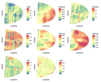
Rather than using the VWC directly, agricultural scientists have begun to use alternative, more easily obtained, data to inform irrigation zones. Examples of such possible data for the Rexburg field considered in this research are shown in Figure 2 and include historical yields, normalized difference vegetation index (NDVI) and elevation (to name a few). These alternative data to VWC were recorded for over 5000 unique locations in the field using simple remote sensing mounted on drones or tractors making these data readily available to farmers.
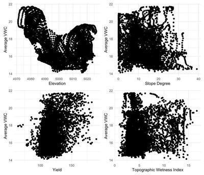
The primary issue of using alternative data to VWC such as that in Figure 2 to define VRI zones is that such data is non-linearly related to VWC and, hence, may result less water efficient zones than ones defined by VWC. Figure 3 below shows scatterplots of a few of the variables against the VWC for the Rexburg field demonstrating clear non-linear relationships. In fact, the scatterplots in Figure 3 show a highly complex relationship between these alternative data and VWC suggesting that zones defined on these data may vary considerably from zones defined on VWC.
The goals of this project and analysis are to use easily to obtain covariates to create irrigation zones that are related to VWC, while accounting for the spatial correlation that exists in the field and modeling the complex relationship that exists between the covariates and VWC. The proposed model integrates deep learning into a statistical modeling framework for irrigation zones to capture the complex relationship between the covariate data and the response variable.
Proposed Model
Deep learning is a subfield of machine learning focused on using highly flexible algorithms called neural networks to learn complex relationships between covariates and response variables. However, from a statistical perspective, deep learning algorithms do not inherently account for uncertainty in the predictions and are often so complex that they are uninterpretable. The model proposed embeds a deep neural network into a statistical model and estimates associated parameters using a Bayesian paradigm allowing for uncertainty quantification in the resulting fit. Further, we implement Bayesian versions of partial dependence plots to give some interpretability to the deep neural network between the covariates and the response variable.
With a deep neural network accounting for the complex relationships between the covariates and response, our model also creates smooth irrigation zones by incorporating spatial correlation into our model. Specifically, we use spatial basis functions distinctly from the neural network portion of the model thereby successfully merging deep learning into a spatial modeling framework. Additionally, the spatial basis functions increase computational efficiency of the Markov chain Monte Carlo algorithm to sample from the posterior distribution of all model parameters.
The primary quantity of interest in this research is the irrigation zone of each location on the field - not necessarily the VWC. Admittedly, we could predict the VWC first and then create irrigation zones by splitting based on predicted VWC quantiles. However, here we first delineate zones based on the quantiles of the observed VWC and then perform modeling for the associated zone. Figure 4 below shows the discretized zones, which represents our response variable.
While this represents loss in information for VWC, we advocate discretizing the response in this way for a few reasons. First, our data is unique in that we have the exact VWC measurements. However, given the cost, obtaining exact VWC data is exceptionally rare in agricultural practice. Rather, most agriculture fields are able to only collect ambiguous VWC levels of “low” or “high.” By transforming our response variable from VWC to irrigation zone, our statistical model will be more aligned with typical data available in other crop fields. That is, by discretization, exact VWC need not be recorded to follow this same methodology to delineate irrigation zones in other fields and our research will be more widely applicable.
Second, VRI technology is typically done by applying “less than average” water to some locations and “more than average” to others. Hence, what is required to implement VRI is knowledge of which locations are “low” and which are “high” rather than the exact VWC.
Given the discretization here to irrigation zones corresponding to VWC levels, the response variable is thus an ordered multinomial response. Under this discretization, we build our model using a latent variable approach to facilitate Bayesian computation. While others have developed statistical models for neural networks, to our knowledge, this is the first attempt at building a deep spatial statistical model for a non-Gaussian response.
The next sections will outline the model that is used and how the parameters were estimated, followed by the results of the model and the conclusions that can be drawn from it.
Model Specification
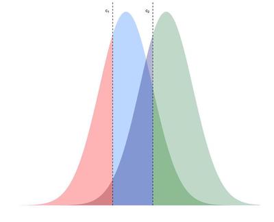
Let $Y(\mathbf{s}) \in {1,\dots,R}$ denote the irrigation zone for location $\mathbf{s} = (s_1, s_2)' \in \mathbb{R}^2$ where $R$ is the number of desired irrigation zones for a field. Given the current state of variable rate irrigation systems, usually $R$ will only be as high as 4 or 5. Due to the difficulty of performing spatial analysis on a discrete scale, we augment $Y(\mathbf{s})$ with a latent variable $Z(\mathbf{s}) \in \mathbb{R}$ such that
\begin{align} Y(\mathbf{s}) = \sum_{r=1}^R r {1}(c_{r-1} \leq Z(\mathbf{s}) < c_{r}) \label{responseMod} \end{align}
where ${1}(\cdot)$ is an indicator function and $c_0 = -\infty < c_1 = 0 < c_2< \dots < c_R = \infty$ are cut points used to determine the probability that location $\mathbf{s}$ belongs to a specific zone.
Figure 5 below illustrates the benefit of using the latent variable, $Z(\mathbf{s})$. The cut points, $c_1$ and $c_2$, are the same for each location, but the probabilities of being in a specific zone are different depending on the mean of $Z(\mathbf{s})$, so the probabilities of being in each irrigation zone is different for each location.
With this specification, we can assume that \begin{align} Z(\mathbf{s}) &\sim \mathcal{N}\left(f_L(\mathbf{X}(\mathbf{s})) + w(\mathbf{s}), 1\right) \label{latentMod} \end{align}
where $f_L(\mathbf{X}(\mathbf{s}))$ is the univariate output function of an $L$-layer feed forward neural network (FFNN) with input covariates $\mathbf{X}(\mathbf{s}) = (X_1(\mathbf{s}),\dots, X_P(\mathbf{s}))'$ and $w(\mathbf{s})$ is a spatial random effect.
This specific model is used because it accounts for the challenges previously mentioned. The FFNN can model the complex relationship between the covariates and the associated irrigation zones and the spatial random effect, $w(\mathbf{s})$, smoothes the predicted zones so they can be implemented by VRI.
A FFNN with $L$ layers, consists of three different types of layers: an input layer, hidden layers and an output layer each consisting of a different number of units. More succinctly, let $(\mathbf{X}(\mathbf{s})) = (f_{l1}(\mathbf{X}(\mathbf{s})),\dots,f_{lP_l}(\mathbf{X}(\mathbf{s}))$ be the vector of $P_l$ units at layer $l$ of the FFNN. The transformation from layer to layer occurs via
$$f_{l}(\mathbf{X(\mathbf{s})}) = a_l(\mathbf{\lambda}_{{l-1}0} + \Lambda_{l-1}\mathbf{f}_{l-1}(\mathbf{X}( \mathbf{s})))$$
where $a_l(\cdot)$ is a element-wise nonlinear activation function used at layer $l$, $(\lambda_{(l-1)01},$ $\dots,\lambda_{(l-1)0P_l})'$ = $\mathbf{\lambda}_{{l-1}0}$, which is the vector of intercepts (biases) applied to layer $l-1$. $\mathbf{\Lambda}_{l-1} = ({\lambda_{(l-1)ij}})_{i,j}$ is the $P_l \times P_{l-1}$ matrix of coefficients (weights) used to transition from layer $l-1$ to layer $l$. For the input layer (i.e.\ $l=1$), we take $\mathbf{f}_1(\mathbf{X}(\mathbf{s})) = \mathbf{X}(\mathbf{s})$ such that $P_1 = P$ is the number of covariates included in the model.
From a statistical point of view, the biases and weights (intercepts and coefficients) are the model parameters to be estimated from the data while the number of layers $L$, the layer dimensions ${P_l}$ and the activation functions are known as tuning parameters and are fixed via cross-validation to optimize prediction performance.
While $f_L(\mathbf{X}(\mathbf{s}))$ captures the non-linear relationship between the response and covariates, the spatial random effect $w(\mathbf{s})$ serves to smooth the predicted zones over space. To achieve this smoothing, we opt to use the Moran basis function expansion for $w(\mathbf{s})$. The number of Moran basis functions used in the model is denoted by $K$. Generally, as $K$ increases then the associated fitted spatial surface from the Moran basis is more variable. Hence, for purposes of this research, we treat $K$ as an additional tuning parameter that we will choose via cross-validation.
Parameter Estimation
Even though neural networks are typically fit via loss minimization, in an effort to merge machine learning and statistical modeling, we adopt a Bayesian approach for parameter estimation to ensure that our predicted irrigation zone surface accounts for associated parameter uncertainty. Accounting for uncertainty here is important so that the predicted irrigation zones can be potentially altered to more easily be incorporated into a VRI system. For example, if zone assigned to a certain location is highly uncertain, then that location can be manually assigned to a zone by the farmers to increase the overall efficiency of the VRI.
Under the Bayesian approach, prior distributions are required for all the neural network parameters ($\mathbf{\lambda}_{l0}$, $\mathbf{\lambda_l}$), the Moran basis coefficients $(\mathbf{\beta})$ and the cut points $c_2,\dots,c_R$ and parameter estimation is done via posterior inference. Because the $\mathbf{\beta}$ parameter vector is simply coefficients in an ordered probit regression model, we assume a vague $N(0, 100\mathbf{I})$ prior distribution because the data can generally estimate these parameters well. Because the cut points are ordered so that $0 < c_2 < \cdots < c_R = \infty$, each cutpoint was transformed according to $c_2^\star = \log(c_2)$ and
\begin{equation} c_r^\star = \text{log}(c_r - c_{r-1}) \end{equation}
for $r=3,\dots,R-1$ and a $\mathcal{N}(0, 10)$ prior was used for each $c_r^\star$. The corresponding back transformation $c_r = \sum_{i=2}^r\exp{c_i^\star}$ ensures the ordering constraint.
The priors for the FFNN weights ${\Lambda_{l}}$ and biases ${\lambda_{0l}}$ need to be chosen with care to avoid overfitting. Neural networks are overparameterized and can easily overfit training data resulting in poor predictive performance. One common approach for restricting neural networks is via penalization (regularization). In a Bayesian setting, regularization is enforced via informative prior constraints. As such, we assume \textit{a priori} independent $\mathcal{N}(0, 0.01)$ priors for all biases and weights. The highly informative $0.01$ variance constrains the biases and weights to be near zero; thus preventing overfitting similar to ridge and LASSO regression models. For our purposes, the above Gaussian prior worked adequately to prevent overfitting.
Posterior inference for our model parameters was accomplished by using Markov chain Monte Carlo (MCMC) sampling. Conditional on all other parameters, the complete conditional distribution for $Z(\mathbf{s})$ is a truncated Gaussian distribution with mean $f_L(\mathbf{X}(\mathbf{s})) + \mathbf{b}'(\mathbf{s})\mathbf{\beta}$, variance 1 and endpoints $c_{Y(\mathbf{s})-1}$ and $c_{Y(\mathbf{s})}$. Because each $Z(\mathbf{s})$ is conditionally independent, this sampling can be done independently and efficiently. Next, because $Z(\mathbf{s}) \in \mathbb{R}$, we use assume $a_L(\cdot)$ is the identity activation and $P_L = 1$ so that \begin{align} Z(\mathbf{s}) \overset{iid}{\sim} \mathcal{N}(\lambda_{0(L-1)} + \mathbf{f}_{L-1}'(\mathbf{X}(\mathbf{s}))\mathbf{\Lambda}_{L-1} + \mathbf{b}'(\mathbf{s})\mathbf{\beta}, 1) \end{align}
which can be rewritten simply as $Z(\mathbf{s}) \sim \mathcal{N}(\mathbf{X}_\star'(\mathbf{s})\mathbf{\beta}^\star, 1)$ where
$$ \mathbf{\beta}^\star = (\lambda_{0(L-1)}, \mathbf{\Lambda}_{L-1}', \mathbf{\beta}')'$$ $$ \mathbf{X}_\star(\mathbf{s}) = (1, \mathbf{f}_{L-1}'(\mathbf{X}(\mathbf{s})), \mathbf{b}'(\mathbf{s}))'$$
Under the above Gaussian priors, the complete conditional for $\mathbf{\beta}^\star$ is Gaussian and can be sampled directly.
While ${Z(\mathbf{s})}$ and ${\lambda_{0(L-1)}, \mathbf{\Lambda}_{L-1}, \mathbf{\beta}}$ can be sampled directly from the corresponding complete conditional distributions, the cut points $c_2,\dots,c_{R-1}$ and other FFNN parameters ${\mathbf{\lambda}_{0l}, \mathbf{\Lambda}_l}_{l=1}^{L-2}$ need to be sampled indirectly via Metropolis-Hastings or other algorithms. The final MCMC algorithms sampled the neural net weight matrix $\mathbf{\Lambda}_{l}$ and the biases $\mathbf{\lambda}_{0l}$ jointly for each layer (with each layer being sampled separately). For our MCMC algorithm, we used the adaptive Metropolis algorithm to update the proposal variance and achieve better mixing for the FFNN parameters. Finally, this adaptive Metropolis algorithm was again used to sample the transformed cutpoints $c_2^\star,\dots,c_{R-1}^\star$ after marginalizing out $Z(\mathbf{s})$.
Results
This sections outlines identified irrigation zones from the model previously defined when fit to the Rexburg field data. For our application, we used the following ten covariates: elevation, yield, NDVI index for 2018 and 2019, two different measures of slope at a location, the $x$ and $y$ aspect of a location, a covariate called analytical, which was an additional measure of aspect and a topographical wetness index. Each of these covariates were observed via remote sensing at 5062 locations in the field.
Model Settings and MCMC Diagnostics
For our implementation, we set the number of irrigation zones, $R$, to 3. As previously mentioned, $R$ will rarely if ever be higher than 4 or 5 and, in discussion with the farm owner, 3 zones was determined to be reasonable based on the field’s VRI capacities. We also used rectified linear unit activation functions for all the activation functions with the exception of the output layer which was an identity activation to match the support of $Z(\mathbf{s})$. Certainly, other activation functions could be used but the rectified linear units is one of the most common.
Beyond the above model settings, implementation of our spatial neural network model requires tuning the number of layers ($L$), the number of units per layer (${P_l}$), and the number of Moran basis functions ($K$). For each parameter setting in Table 1, we implemented a 6-fold cross validation and averaged the adjusted Rand index across the 6 folds as a predictive performance metric. Prior to fitting the models in Table 1, a larger grid was first used to get a general idea of the reasonable values for the tuning parameters. Given our data set consisted of only 66 observations, an effort was made to keep the total number of parameters for the model less than 25 to prevent overfitting. Deeper neural networks, generally, require a lot of data to be effective. Hence, the grid search only examines one or two layer neural networks (in addition to the input and output layers). The maximum number of Moran basis functions considered was 10 in order to make sure that the zones were being determined by the neural network predictions rather than being overly driven by the spatial aspect of our model.
Table 1 shows the cross validation results and finds that a single layer with 10 neurons and 5 Moran basis functions were the ideal parameters for this data. The results displayed in the following subsections are from this model setting. Note that, generally, from Table 1, adding spatial basis functions improved the model’s predictive ability suggesting that novel contribution of merging spatial modeling techniques with deep learning is of value in this particular setting.
Neurons |
Layers |
Spatial |
Rand Index |
|---|---|---|---|
| 10 | 1 | 0 | .06767 |
| (10,10) | 2 | 0 | .1776 |
| 20 | 1 | 0 | .12296 |
| 10 | 1 | 5 | .31795 |
| (10,10) | 2 | 5 | .22377 |
| 20 | 1 | 5 | .13879 |
Table 1: Cross Validation results. The first column lists the number of neurons for each layer, the second column indicates the number of layers for the neural net, the third column shows the number of Moran basis functions, and the fourth column gives the average adjusted Rand index over the 6 folds
When using Markov chain Monte Carlo sampling in a Bayesian framework as is the case here, it is important to make sure that the algorithm provides samples of the parameters from posterior distribution via convergence diagnostics. Figure 6 display trace plots of $f_L(\mathbf{X}(\mathbf{s})) + w(\mathbf{s})$ for four different locations in the field while Figure 7 displays trace plots of the cut point. We display these trace plots as $f_L(\mathbf{X}(\mathbf{s})) + w(\mathbf{s})$ and the cut point because they are the main quantities from which we derive our irrigation zone delineation. These trace plots show that these parameters have converged and they can be used to for posterior inference.
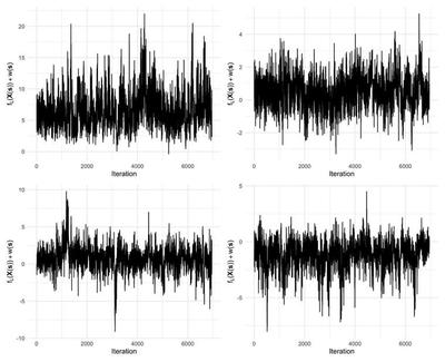
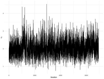
Although we estimated many more parameters, these were the parameters that we were using to make inference, so we were only concerned about convergence for these parameters.
Model Comparisons
As a means to validate the use of the spatial neural network model proposed in this analysis, three additional alternative models were fit to the data and the adjusted RAND index (ARI), a similarity measure between the predicted irrigation zone from the model predictions against the observed irrigation zones, was calculated for the 5062 locations across the field in Rexburg.
The four models compared are ordinal logistic regression with linear effects, ordinal logistic regression with natural splines, the neural network model with no spatial basis functions and our full neural network model with spatial basis functions. The ordinal logistic regression is a common approach to modeling discrete ordinal multinomial response variables. One of the drawbacks is the assumptions that the relationship between predictors and the response is linear. Splines are a common approach to modeling non-linear relationships for statisticians, while neural networks are often a machine learning approach to account for these non-linear relationships. These two models can provide a comparison between these two different approaches to model a non-linear relationship. While neural networks and splines are able to account for the non-linear relationships, they don’t incorporate any spatial correlation. For irrigation zone delineation, the spatial correlation is used to smooth out the irrigation zone predictions across the field. As a result, the fourth model is the neural network with the spatial basis functions to help improve the predictions of the zones.
Model |
Adjusted RAND index |
|---|---|
| Ordinal Logistic Regression | 0.2065 |
| Ordinal Logistic Regression with Natural Splines | 0.2273 |
| Neural Network | 0.2245 |
| Neural Network with Spatial Basis Functions | 0.2741 |
Table 2: RAND index for the four different models for all 5062 locations in the field.
Covariate Effects
One of the drawbacks of using neural network models as we have here is that the parameters have no intuitive interpretation. Although the parameters are not interpretable, partial dependence plots and feature importance can be used to intuitively understand the effects of covariates on the response.
First, partial dependence plots are used to show the marginal effect of a covariate on the predicted outcome. Mathematically, the partial dependence plot for a covariate, say $X_p$ , is calculated as
\begin{align} \text{PDP}(X_p) &= \frac{1}{n}\sum_{i=1}^n \left(\widehat{f}_L(X_p, \mathbf{X}_{-p}(\mathbf{s}_i)) + \widehat{w}(\mathbf{s}_i)\right) \label{pdpeq} \end{align}
where $\mathbf{X}_{-p}(\mathbf{s}_i)$ is the vector of covariates with $X_p(\mathbf{s}_i)$ removed and replaced with a single value (for all observations) of $X_p$ and $\widehat{f}_L(\cdot)$ and $\widehat{w}(\cdot)$ is our fitted spatial neural network model.
The above is calculated for a grid of $X_p$ in the domain of $X_p(\mathbf{s})$ to produce a curve representing the marginal effect of $X_p(\mathbf{s})$. Intuitively, the partial dependence measure is calculated by replacing the variable of interest ($X_p(\vec{s})$) with a single fixed value for all observations in the data and averaging the associated prediction across observations. Because we adopted the Bayesian approach, the uncertainty for these partial dependence plots are accounted for as well via Monte Carlo sampling.
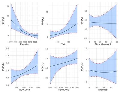
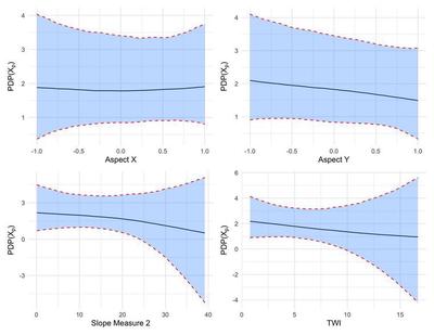
Figures 8 and 9 above show the partial dependence plots for the ten covariates that were used in the analysis where the black line represents the posterior mean of marginal effect for the covariate and the shaded region is the 95% credible interval for the marginal effect. Elevation, yield, and the NDVI for 2018 and 2019 seemed to heavily influence the probability of belonging to an irrigation zone. For example, as elevation increases, the probability of belonging to a lower-water zone increases (Zone 1 corresponds to the zone with the smallest VWC which, in turn, would get the most irrigation to compensate). The other covariates appear to have a minimal effect on the predicted zone.
Another common measure for covariate influence on machine learning models is feature importance. For this analysis, the permutation feature importance was used as the feature importance measure. The feature importance was calculated by permuting values of the feature (covariate) and calculating the ARI for the model with the permuted feature. The purpose of permuting the covariate is to break the relationship between the feature and the response. Under permutation, the predictive accuracy should decrease for features that are highly predictive of the response. After calculating the ARI for the model with the permuted feature, the feature importance for the $p^{th}$ covariate ($X_p(\mathbf{s})$) is calculated as:
\begin{align} FI_p = ARI_{\text{orig}}/ARI_{\text{perm}} \label{FI} \end{align}
where $ARI_{\text{orig}}$ is the ARI for the model before permutation and $ARI_{\text{perm}}$ is the ARI for the model after feature $X_p(\mathbf{s})$ had been permuted. Since ARI is on a scale from -1 to 1, the original ARI was divided by the permuted ARI so that a higher feature importance would correspond to a more important feature.
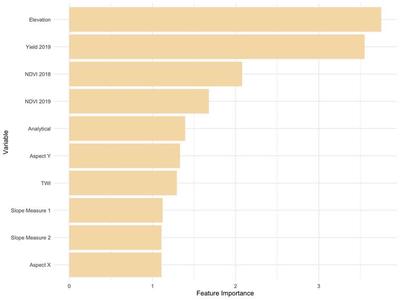
The feature importance plot in Figure 10 above shows the feature importance for the 10 covariates that were included in the model. In correspondence with the partial dependence plots, the results from the feature importance plot also indicates that elevation, yield, and the NDVI index from 2018 and 2019 are important covariates in determining the irrigation zone. Hence, for other agricultural fields where irrigation zones are desired, collecting the most importance features will provide the most effective zones for variable rate irrigation.
Field-wide Irrigation Zone Delineation
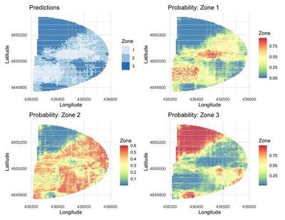
The fitted spatial neural network model was used to make predictions of which irrigation zone a location should be classified in across the whole field. Due to Monte Carlo sampling, the uncertainty in the zone delineation was also able to be calculated. Figure 11 below shows the highest probability zone by location (top left) along with the probabilities of each location being assigned to each of the three zones. The predictions appear to fairly spatially contiguous zones (as desired) with the exception of middle of the field in areas between zone 1 and 2.
While the zone prediction map in Figure 11 produces zones that are spatially smoothed by the spatial basis function, the covariates produce some non-contiguous regions that would be difficult to implement using variable rate irrigation given the current state of precision agriculture. Rather, for VRI implementation purposes, we desire to further smooth the predicted zones into purely contiguous zones. For purposes of VRI implementation, we use a spatial clustering algorithm based on finite differences to achieve more contiguous zones. Specifically, we spatially cluster using ward dissimilarity based on the expected zone \begin{align} E(Y(\mathbf{s})) &= 1\times\left[\Phi(0-\widehat{f}_L(\mathbf{X}(\mathbf{s})) + \widehat{w}(\mathbf{s}))\right] + \notag \newline & 2\times\left[\Phi(\widehat{c}_2-\widehat{f}_L(\mathbf{X}(\mathbf{s})) + \widehat{w}(\mathbf{s}))-\Phi(-\widehat{f}_L(\mathbf{X}(\mathbf{s})) + \widehat{w}(\mathbf{s}))\right] + \notag \newline & 3\times \left[1-\Phi(c_2-\widehat{f}_L(\mathbf{X}(\mathbf{s})) + \widehat{w}(\mathbf{s}))\right] \label{weight} \end{align} where $\Phi(\cdot)$ is the standard normal cumulative density function.
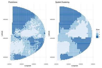
The result from this clustering process is shown in Figure 12 and compared with the original predictions. While there are still some discrepancies between the clustered zones and the original zones, they are relatively similar and the clustering provides contiguous zones that would be viable to be implemented with VRI.
Conclusions
This analysis presents a Bayesian spatial neural network model with easily obtainable predictors such as elevation, slope, and past crop yields to be used for irrigation zone delineation.
We propose this model as an alternative to the expensive and time consuming process of measuring volumetric water content. The model provides a fusion of statistical modeling and deep learning by harnessing the predictive ability of artificial neural networks, while quantifying uncertainty using Bayesian methods and using spatial modeling to capture spatial correlation in the irrigation zones. The analysis showed that for the field in Rexburg, Idaho, the most influential covariates for delineating irrigation zones were elevation, yield and the NDVI index.
There are some issues with the model presented that could be examined to improve upon the proposed model. As mentioned, the neural network weights individually did not converge well. While we used efforts such as strong prior assumptions (the equivalent of penalization in traditional neural network model fitting), we still did not achieve strong mixing properties of the Markov chain desirable for posterior inference. One possible solution to this is to use Hamiltonian Monte Carlo techniques which could integrate the backward-propogation algorithm but in a Bayesian posterior sampling paradigm.
There were 3 irrigation zones chosen for this analysis, but the performance of the model as the number of zones increase has yet to be studied and it is unknown if the model will perform as well when there are more than 3 irrigation zones. Further, perhaps more irrigation zones would increase the efficiency of the VRI technology. Future research could consider the effect of the number of zones on the fitted model.
Finally, the predictions from the model gives zones that are not completely spatially contiguous. For the results to be useful for farmers, they need to have spacial contiguous zones that would be feasible to be implemented with VRI. In this scenario, spatial hierarchical clustering was used to smooth the predictions even further in order to get contiguous zones. There may be other approaches to smoothing out the predictions to get useful irrigation zones that can be implemented with VRI systems.
In addition to the potential issues that should be further studied, there is potential future work that can be done based on the results from the analysis. First, the analysis and results of this model has only been applied to the one field in Rexburg. It would be beneficial to be able to use the model to delineate other fields. The model will be most beneficial when it is portable to other fields and scenarios. At the moment, the efficacy of this model is only known for the field of winter wheat in Rexburg.
In addition, to increase the portability of the model, it would be useful to consider other possible covariates that could be used to determine the volumetric water content. The covariates that were used in the analysis were provided and consequentially there may be other covariates that would be beneficial to delineating irrigation zones. For this analysis, we used ten different covariates and a number of them did not appear to be extremely important in determining the irrigation zone based on the partial dependence and feature importance plots. The impact of adding and subtracting covariates from the model could be examined further.
Overall, the use of Bayesian spatial neural network models has the ability to create accurate irrigation zones from easily obtained data about a field without having to put in painstaking effort to determine the volumetric water content. As a result, these models could make the implementation of variable rate irrigation easier for farmers in agricultural fields.